


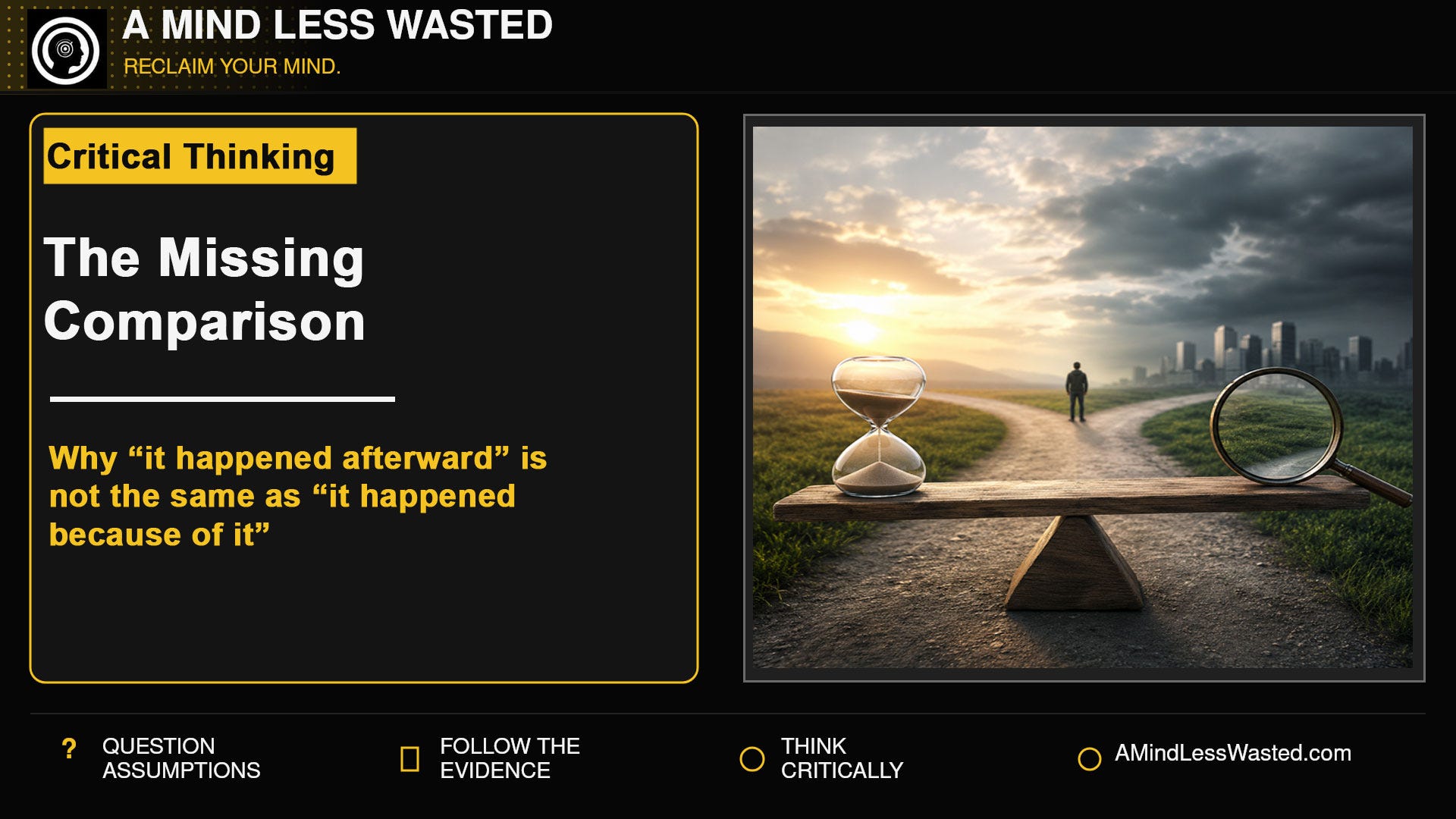
You start taking a remedy on Wednesday, when your symptoms are at their worst. By Friday, you feel much better.
The remedy worked.
Or did it?
There is nothing imaginary about the improvement. You were sick, you took something, and then you recovered. But that sequence alone cannot tell us what the remedy did. Perhaps it helped. Perhaps you would have felt just as good by Friday without it.

Now consider a county that installs speed cameras at dangerous intersections. The following year, casualties decline. Or a hospital that reports three times as many pressure ulcers as another hospital.
The cameras worked. The hospital must be worse.
Again, maybe. But each conclusion goes beyond the fact that supports it. We know what happened. We do not yet know what caused it.
The missing piece is easy to overlook because we can never observe it directly:
What would probably have happened otherwise?
The half of the claim we cannot see
Whenever we say that one thing caused another, we are making an unstated comparison. We are saying the outcome would have been different if the treatment, policy, exposure, or decision had never occurred.
We can observe the first version of events. We cannot rewind Wednesday, skip the remedy, and live through the same illness again. A city cannot adopt a new policy and simultaneously leave that policy unadopted. The same patients cannot receive care at two hospitals under identical circumstances.
Researchers call the unobserved version the counterfactual. Statistician Paul Holland called this the fundamental problem of causal inference: for the same person, place, or group, we cannot observe both the outcome under an intervention and the outcome that would have occurred without it.
That does not mean we can never work out what causes what. It means we need a reasonable substitute for the outcome we cannot see. In a clinical trial, that may be a randomized control group. In a policy evaluation, it may be a similar place where the policy was not introduced. Sometimes researchers use an established trend or a statistical model.
The conclusion is only as reliable as the substitute.
“I took it, and I got better”
Personal experience can be powerful evidence that something happened. It is much weaker evidence for why it happened.
Imagine waiting until your symptoms become unbearable before trying a treatment. This is common. People do not usually reach for a new remedy when they feel average. They try it on a terrible day.
Many symptoms fluctuate. An unusually bad day is often followed by one closer to normal, with or without treatment. This is called regression to the mean. It can make an ineffective remedy appear to have produced a dramatic improvement simply because we started using it when the problem was near its worst. A British Medical Journal discussion explains how easily this can distort medical decisions.
Natural recovery presents the same problem. If an illness usually improves within a week, nearly anything taken on day five may look impressive by day seven. Other care, a change in behavior, or expectations about the treatment may also affect how a person feels or reports symptoms.
None of these possibilities proves the remedy did nothing. They show why the sequence itself is not enough.
This is one reason clinical trials use control groups. According to FDA guidance, a control helps separate the effect of a treatment from the natural course of the illness, expectations, other care, and outside influences.
The choice of control also determines the question the trial can answer. A treatment may appear to help when compared with receiving nothing, yet perform no better than a placebo. It may beat a placebo but offer no meaningful advantage over the standard treatment patients already receive.
Those results can all be accurate. They are comparisons with different meanings.
What happened after the policy?
The same problem appears whenever a result is measured before and after a decision.
A new law takes effect, and crime falls. A school adopts a curriculum, and test scores rise. A company hires a new executive, and profits improve.
The timing matters. It may even be our first clue that the decision had an effect. But what if the trend had already begun? What if the economy changed, another policy took effect, or the unusually bad year that prompted the intervention was unlikely to repeat?
A before-and-after comparison tells us what changed. By itself, it usually cannot tell us how much of that change was caused by the intervention. The World Bank makes this distinction in its guide to impact evaluation. Last year’s result is not automatically a good estimate of what would have happened this year.
A real speed-camera evaluation in North Yorkshire shows why this matters.
Researchers examined 22 locations where mobile safety cameras had been introduced. Casualties fell from 46 before the cameras to 33 afterward, a decline of 13.
It would be tempting to credit the cameras with all 13. The cameras arrived. The number fell.
But these locations had been selected because they were collision hotspots. Their unusually high casualty count may have included a temporary spike. Casualties were also falling more broadly.
Using earlier trends and control sites, the researchers estimated that casualties would have declined from 46 to about 41 even if the cameras had not been introduced. Their model attributed about 4.5 of the decline to regression to the mean and another 0.5 to the broader trend. The model attributed the remaining reduction, eight casualties, to the cameras. The North Yorkshire evaluation described this as an estimated 20 percent effect.
The fairer comparison did not erase the apparent benefit. It reduced it to a more believable estimate.
That estimate is not the final word. It depends on the model and on whether the control locations were sufficiently similar. Researchers still could not visit an alternate North Yorkshire where the cameras were never installed.
But they did much more than assume that every casualty avoided after the cameras appeared was avoided because of them.

“Compared with what?” is a question, not a rebuttal
Asking for a fair comparison does not show that a claim is false. Sometimes the claim survives and becomes more convincing. The point is to find out how much of the result the evidence can reasonably support.
Two groups are not necessarily a fair comparison
Sometimes a comparison is plainly visible but still gives the wrong impression.
The Agency for Healthcare Research and Quality offers a useful example involving pressure ulcers at two hypothetical hospitals. Hospital A recorded 20 cases for every 1,000 eligible patients. Hospital B recorded 60.
Hospital B appears to be doing three times worse.
The patients, however, were very different. Based on age, diagnoses, and other health conditions, Hospital B was expected to have 100 cases per 1,000 patients. Hospital A was expected to have 40.
After risk-adjusting the results to the same reference rate, AHRQ calculated rates of 25 per 1,000 for Hospital A and 30 for Hospital B. Hospital A still did slightly better, but the apparent threefold gap nearly disappeared. Both hospitals had fewer cases than expected for the patients they treated. The calculation is included in the AHRQ Quality Indicators Toolkit.
The original rates were correct. They told us what happened among the patients at each hospital. They could not tell us how the hospitals would compare if they treated similar patients.
Age can distort population comparisons in much the same way. A state with an older population may have a higher overall death rate even if the risk at each age is no higher. The CDC uses age adjustment to make those comparisons fairer.
We also need to consider how outcomes were found. A group that sees doctors more often or undergoes more testing has more chances to receive a diagnosis. More recorded illness could mean more actual illness, more opportunity to find it, or both. Cochrane identifies unequal methods or intensity of observation as a source of detection bias.
Even a perfectly counted number can mislead if the denominator is wrong. A group of one million people may produce more cases than a group of ten thousand while posing much less risk to each person. Raw counts tell us about total burden. Rates are usually more useful when we are comparing risk. The CDC’s Field Epidemiology Manual explains why rates must account for population size and observation time.
Adjustment helps, but it cannot make two groups identical. Researchers can account only for differences they measured and modeled well. Adjusting for the wrong variable can even introduce bias.
Risk adjustment improves a comparison only to the extent that the model includes the relevant differences and represents them accurately.
So the word adjusted should not end our questions. We still need to ask whether the analysis addressed the differences most likely to distort that particular comparison.
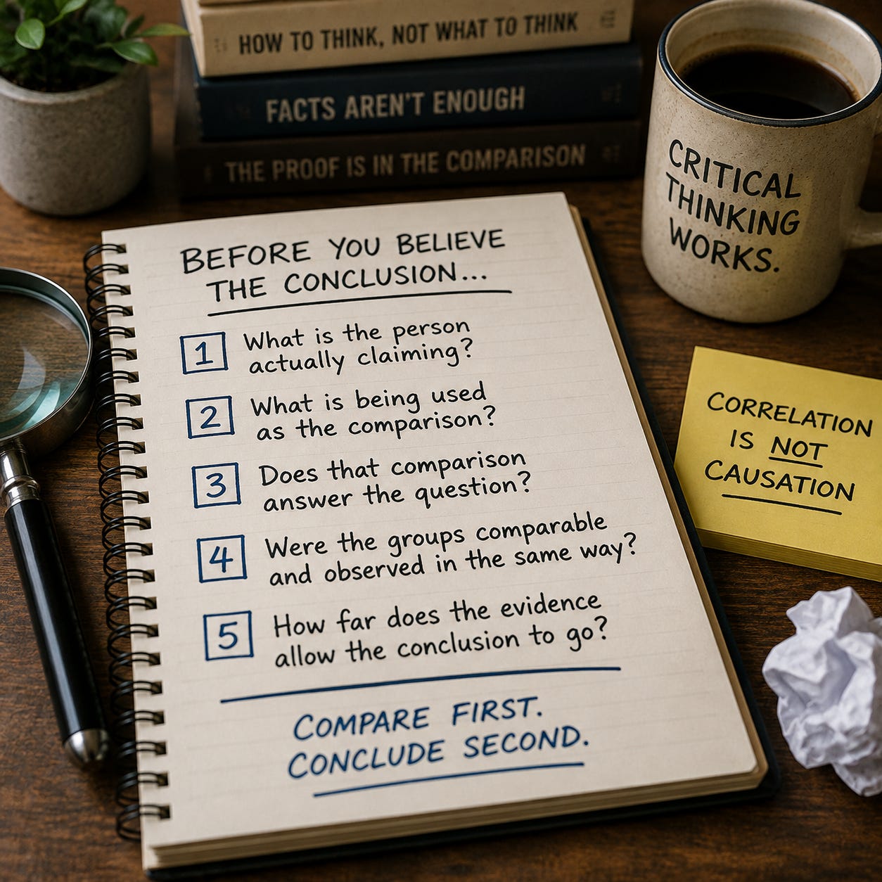
A five-question comparison check
You do not need to recreate a statistical analysis every time you encounter a causal claim. These five questions will catch many of the most common problems.
1. What is the person actually claiming?
“Deaths fell last year” describes what happened. “This policy caused deaths to fall” tries to explain why.
The explanation carries a greater burden of proof.
2. What is being used as the comparison?
Is a treatment being compared with no treatment, a placebo, or standard care? Is this year being compared with last year? Are two different populations being placed side by side?
If the comparison is never stated, the conclusion may rest entirely on timing or assumption.
3. Does that comparison answer the question?
Beating a placebo does not show that a treatment is better than existing care. A raw number of cases cannot tell us which group faced the greater individual risk. An earlier year may be a poor guide to what would have happened this year.
4. Were the groups comparable and observed in the same way?
Look for differences in age, health, disease severity, earlier trends, access to care, follow-up time, and opportunities to detect the outcome.
Any of them may create part or all of the apparent effect.
5. How far does the evidence allow the conclusion to go?
A weak comparison does not prove the proposed cause had no effect. It means the evidence has not separated that effect from the alternatives.
The honest conclusion may be possible, suggestive, or associated with rather than proved or caused.
Where the mistake happens
Misleading arguments do not always depend on invented statistics. Often the number is accurate, the event happened, and the person reporting it is sincere.
The mistake comes in the jump from observation to explanation.
You took the remedy, and you improved. That tells us what happened to you. It does not tell us how you would have felt without it.
Casualties fell after the cameras were introduced. The decline was real. The raw number alone could not tell us how much credit the cameras deserved.
One hospital reported more complications. That may be important for planning and patient care. It does not establish that the hospital provided worse care to comparable patients.
Critical thinking begins by noticing when a fact has quietly become a causal claim. Before accepting the explanation, ask what evidence separates it from the other possibilities.
Compared with what would probably have happened otherwise?
If this article changed how you think about evidence, subscribe to A Mind Less Wasted. Each week you'll get practical critical thinking tools, fact checks, and evidence-based articles that help separate strong arguments from persuasive ones.
Resources and Further Reading
Paul W. Holland, “Statistics and Causal Inference”
A foundational paper explaining why causal inference requires comparing an observed outcome with a potential outcome that cannot also be observed for the same person or unit.
FDA and ICH, “E10: Choice of Control Group and Related Issues in Clinical Trials”
Explains the purposes of placebo, active-treatment, no-treatment, dose-response, and external control groups, and how the choice of control affects what a trial can establish.
Veronica Morton and David J. Torgerson, “Effect of Regression to the Mean on Decision Making in Health Care”
A concise explanation of how selecting patients when their symptoms are unusually severe can make later improvement appear to be a treatment effect.
World Bank, Impact Evaluation in Practice
Explains counterfactual reasoning in policy and program evaluation and why simple before-and-after comparisons are often unreliable.
North Yorkshire, “The Evaluation of Mobile Road Safety Cameras”
The speed-camera evaluation discussed in this article, including estimates for regression to the mean, broader casualty trends, and the camera effect.
Agency for Healthcare Research and Quality, AHRQ Quality Indicators Toolkit
Includes the hypothetical hospital example showing how patient differences can greatly reduce an apparent performance gap after risk adjustment.
CDC, “Age Adjustment”
Explains why crude rates can mislead when populations have different age structures.
Cochrane Handbook, “Assessing Risk of Bias in a Non-Randomized Study”
Discusses detection bias and other problems that can arise when groups are observed or assessed differently.
CDC, Principles of Epidemiology in Public Health Practice
A practical guide to counts, risks, rates, denominators, and person-time in epidemiologic comparisons.
If this article gave you a useful way to test claims about treatments, policies, and group differences, subscribe to A Mind Less Wasted for more evidence-based fact-checks and critical-thinking tools.
And if you know someone who has ever confused “it happened after” with “it happened because of,” share this article with them.
I kept the structure and voice intact while folding in only the accuracy edits that materially improved it.